summary
Genomics experiments have numerous sources of both technical and biological variation
that can confound analysis and interpretation. Therefore, one of the most important steps
in genomics data analysis is generating high-level summary stats of one’s data to ask if the
basic observations align with the expectation. Doing such quality control as early
as possible in the analysis workflow helps to head off unnecessary time spent chasing
technical artifacts that masquerade as biological signals. This quality control
is the motivation behind the bedtools summary command.
Given an input interval file in standard formats, as well as a genome file defining
the chromosome names and lengths relevant to your data, bedtools summary will compute
several summary statistics detailing, for each chromosome, the number of intervals,
the total number of base pairs, and the fraction of intervals and base pairs observed
in your input file. From these summary measures, one can get a quick sense of questions like:
- Are all chromosomes represented in my data or annotation file?
- Do all chromosomes have the expected number of intervals or fraction of base pairs represented?
- Which chromosomes are outliers?
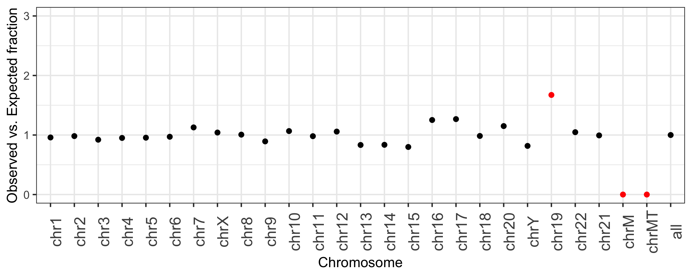
For example, the following plot was generated directly from the output of bedtools summary.
It depicts, for each chromosome, the fraction of all intervals in the RepeatMasker track from UCSC
observed on each chromosome versus the fraction of RepeatMasker intervals that are expected
for each chromosome, based on the fraction of the genome that each chromosome represents.
This plot highlights that chr19, chrM, and chrMT (the different mitochondrial reference genomes) are outliers.
Chromosome 19 has more than 1.5 times the intervals that are expected based upon the length of
the chromosome. ChrM has no intervals, making the observed-to-expected ratio be 0.
This former is because the repeat content of chromosome 19 “is approximately 55%, more than 10% higher
than the genome-wide average” (Grimwood J, et al. Nature. 2004;428:529–35). The latter is because
are indeed no repeat annotations provided by UCSC for the mitochondrial genome.
In this case, the extremes in observed versus expected ratios make sense. However, this tool allows one to detect cases that do not and are either artifacts or biological signals.
Default behavior
bedtools summary scans the input interval file and the chromosome lengths provided in
the “genome” file and reports the following columns for each chromosome.
- chrom (chromosome name)
- chrom_length (the length of the chromosome in bp)
- num_ivls (the total number of intervals observed for the chromosome)
- total_ivl_bp (the total number of bp observed in the intervals for the chromosome)
- chrom_frac_genome (the fraction of the genome represented by the chromosome)
- frac_all_ivls (the fraction of all intervals observed the chromosome)
- frac_all_bp (the fraction of all bp observed the chromosome)
- min (the smallest interval observed on that chromosome)
- max (the largest interval observed on that chromosome)
- mean (the mean interval length observed on that chromosome)
In addition, bedtools summary reports a final line with the chromosome name “all”, which
depicts the metrics above but tabulated across all chromosomes in the input file.
As an example, let’s recreate the figure above by running bedtools summary on the
simple repeats track from UCSC. We’ll begin by downloading the data in track the
track table and converting it to BED format.
curl -s http://hgdownload.soe.ucsc.edu/goldenPath/hg38/database/simpleRepeat.txt.gz  \
    | gzcat \
    | cut -f 2-5 \
    | grep -v -E 'Un|fix|random|alt|hap' \
    > simrep.grch38.bed

head simrep.grch38.bed
chr1        10000   10468   trf
chr1        10627   10800   trf
chr1        10757   10997   trf
chr1        11225   11447   trf
chr1        11271   11448   trf
chr1        11283   11448   trf
chr1        19305   19443   trf
chr1        20828   20863   trf
chr1        30862   30959   trf
chr1        44835   44876   trf
Now, let’s make a “genome” file for GRCh38 from the chromInfo table at UCSC
curl -s http://hgdownload.soe.ucsc.edu/goldenPath/hg38/database/chromInfo.txt.gz \
    | gzcat \
    | cut -f 1-2 \
    | grep -v -E 'Un|fix|random|alt|hap' \
    > grch38.genome.txt

head grch38.genome.txt
chr1        248956422
chr2        242193529
chr3        198295559
chr4        190214555
chr5        181538259
chr6        170805979
chr7        159345973
chrX        156040895
chr8        145138636
chr9        138394717
Now, let’s run bedtools summary.
bedtools summary -i simrep.grch38.bed -g grch38.genome.txt | column -t
chrom  chrom_length  num_ivls  total_ivl_bp  chrom_frac_genome  frac_all_ivls  frac_all_bp  min  max     mean
chr1   248956422     74548     15557884      0.080613126        0.077210928    0.048725518  25   124438  208.696195740
chr2   242193529     74474     14493548      0.078423273        0.077134284    0.045392139  25   336509  194.612186803
chr3   198295559     56894     13946854      0.064208928        0.058926309    0.043679955  25   500000  245.137518895
chr4   190214555     56685     10160257      0.061592265        0.058709844    0.031820766  25   136950  179.240663315
chr5   181538259     53887     16801740      0.058782844        0.055811896    0.052621133  25   500000  311.795794904
chr6   170805979     51802     11222841      0.055307687        0.053652418    0.035148658  25   500000  216.648797344
chr7   159345973     55972     20054618      0.051596890        0.057971375    0.062808775  25   150228  358.297327235
chrX   156040895     50432     27398336      0.050526692        0.052233481    0.085808462  25   500000  543.272842640
chr8   145138636     45937     15650021      0.046996495        0.047577915    0.049014080  25   500000  340.684437382
chr9   138394717     39329     10932158      0.044812786        0.040733870    0.034238272  25   159861  277.966843805
chr11  135086622     41279     14127024      0.043741611        0.042753526    0.044244227  25   500000  342.232709126
chr10  133797422     45074     11407694      0.043324163        0.046684087    0.035727596  25   110000  253.088121755
chr12  133275309     44151     13878240      0.043155100        0.045728117    0.043465064  25   356015  314.335802134
chr13  114364328     29907     9423815       0.037031646        0.030975307    0.029514313  25   110000  315.103989033
chr14  107043718     27973     9245970       0.034661202        0.028972223    0.028957323  25   173523  330.531941515
chr15  101991189     25557     9565023       0.033025172        0.026469921    0.029956561  25   110000  374.262354736
chr16  90338345      35288     11959674      0.029251932        0.036548522    0.037456334  25   138208  338.916175470
chr17  83257441      32093     16264416      0.026959106        0.033239393    0.050938295  25   132210  506.790141152
chr18  80373285      23966     18684937      0.026025204        0.024822089    0.058519091  25   500000  779.643536677
chr20  64444167      22608     12620160      0.020867290        0.023415580    0.039524901  25   500000  558.216560510
chr19  58617616      30854     11391752      0.018980628        0.031956135    0.035677667  25   396802  369.214753355
chrY   57227415      15130     4564760       0.018530475        0.015670458    0.014296307  25   227093  301.702577660
chr22  50818468      16760     10691540      0.016455232        0.017358684    0.033484683  25   498537  637.920047733
chr21  46709983      14911     9253172       0.015124887        0.015443636    0.028979879  25   499939  620.560123399
chrM   16569         0         0             0.000005365        0.000000000    0.000000000  -1   -1      -1
all    3088286401    965511    319296434     1.0                1.0            1.0          25   500000  330.702015824
Notice the following:
- There are 0 intervals reported for chrM or chrMT; therefore, the min, max, and mean are all “-1”.
- The last line in the output is has an “genome” chromosome, meaning it is a summary of all of the chromosomes.
Using this report, there are many high-level sanity checks one can explore. For example, we can create the plot described above by saving the output to a file.
bedtools summary -i simrep.grch38.bed -g grch38.genome.txt > ~/simrep.summary.tsv
Now run following R code. (Sorry, I am not an R expert)
if (!require("dplyr")) install.packages("dplyr")
if (!require("ggplot2")) install.packages("ggplot2")
library(dplyr)
library(ggplot2)

x = read_tsv('~/simrep.summary.tsv')
x = x %>% mutate(obs_v_exp = frac_all_ivls/chrom_frac_genome)

p = ggplot(x) +
ylim(0,3) +
ylab("Observed vs. Expected fraction") +
xlab("Chromosome") +
geom_point(aes(x=factor(chrom, level=chrom),
                y=obs_v_exp,
                color=ifelse(obs_v_exp>1.5 | obs_v_exp<0.5, 'red', 'black'))) +
scale_color_identity() +
theme_bw()
p + theme(axis.text.x = element_text(size = 12, angle = 90))